LLM Serving Optimization Starts With an Analytical Floor

A slow time per output token can mean five different things: a fundamental bandwidth limit, an implementation gap, exposed communication, host overhead, or a bad kernel. Most teams find out which one by opening a profiler and grinding through benchmarks. A new paper on arXiv proposes a cheaper first move: compute an analytical floor for your serving configuration before you profile anything, then let the gap between measurement and floor tell you where to look.

The methodology is called Floor First, and it ships as a zero-dependency artifact - a floor calculator plus an agent skill you can wire into automated optimization loops. The core idea is simple enough to sketch: model each decode step as a five-dimensional resource vector (HBM bytes, FLOPs, network bytes, network messages, KV capacity), sum the terms that share a resource, take the maximum across independent resources, and you get two numbers - an optimistic floor and a no-overlap floor. Any benchmark that lands inside that [max, sum] interval is already telling you how much overlap your system is getting before you've opened a single profiler.

Why Your Parallelism Layout Is a Computation, Not a Preference

The paper's case study is where this stops being abstract. DeepSeek-family models have been deployed with opposite attention layouts on comparable hardware: the official DeepSeek deployment decodes with large-scale expert parallelism and data-parallel attention (a layout vLLM's default recipe also enables), while a production 2x8 H20 cluster serves DeepSeek-V3.2 with plain TP16 attention - the historical default for serving frameworks. Nobody in the existing reports derives the choice from an explicit resource account, and none can say at what concurrency the answer flips.

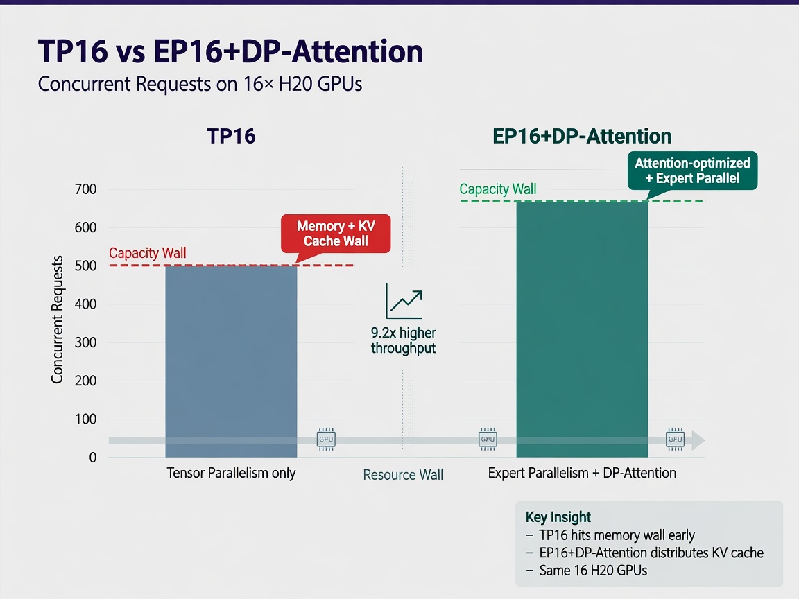
Floor First can. On 16 NVIDIA H20 GPUs - memory-rich and compute-poor, so decode should exploit bandwidth - TP16 decoding at batch 64 and 8K context is KV-capacity-limited to roughly 70 concurrent requests. An EP16 + DP-attention layout trades slightly worse same-batch weight traffic for an order-of-magnitude higher capacity wall of about 644 requests. Same hardware, same model; the right answer depends on your operating point. That's why teams shipped opposite layouts without either being wrong.

The arithmetic behind it is the ridge-point comparison: decode at batch 64 runs at workload arithmetic intensity of roughly 11 FLOP/byte against an H20 ridge point of about 74 (versus roughly 590 on an H100). When MBU hits 80%, MFU sits at 12% - which is exactly why the paper's metric-selection principle matters: report MBU for bandwidth-bound decode and MFU for compute-bound prefill, whichever ceiling is actually binding.

The Benchmark Rules That Make Any of This Usable

A floor is only useful if the measurements you compare against it mean something. The paper lays out four rules for benchmarks feeding this workflow: open-loop load generation (closed-loop generators issue the next request only after the previous completes, so an overloaded system receives less load and tail latency looks artificially healthy), realistic length distributions, steady state before measuring, and tail percentiles rather than averages.

That closed-loop trap alone justifies reading this piece if you've ever quoted a capacity number from a benchmark script - capacity claims without open-loop load generation are meaningless. And without an explicit target stated up front (TTFT? TPOT? goodput against an SLO?), benchmark numbers aren't even partially ordered; you can't tell whether config A beat config B in any way that matters.

The workflow itself: build the floor first, read every benchmark as a residual against it. Small residual - stop investigating. Large residual - now profiling has a specific job: check whether time is missing between kernels, whether communication got exposed, or whether one kernel class blew its analytical budget.

Where This Actually Gets Used Day to Day

Here's my read on what matters most here: the paper explicitly calls out LLM coding agents as where this gap bites hardest, because their default optimization behavior is precisely the loop Floor First warns against - benchmark many configs, open heavy profilers when latency misses a target. If you're running agentic optimization loops over serving configs today (and plenty of teams are), this gives you something enforceable rather than advisory: compute the floor before burning GPU hours on grid search over parallelism layouts.

Two honest caveats from my own read of what's here. First, this isn't validated end-to-end yet - the measurement campaign and residual sweep are planned but not performed in this paper; you'd be adopting the methodology on analytical arguments plus one case study until those land. Second, I'd expect real production workloads to strain the compositional model at its edges: sparse attention variants like DSA-style approaches remove KV-bandwidth terms but leave KV-capacity walls intact exactly as modeled here - that part holds up cleanly in analysis but I'd want to see it confirmed under real traffic distributions before trusting floors as stopping criteria rather than starting points.

What I'd actually do with this: wire the calculator into any prefill/decode disaggregation decision before touching CUDA graphs or kernel tuning again.